Have you ever wondered why the 10th turn of a conversation with an LLM feels just as fast as the first? Mathematically, this shouldn’t happen. As the context grows (History + New Question), the computation required to generate the next token should increase linearly. The secret sauce is KV Cache (Key-Value Cache). It is the single most critical component in LLM Inference optimization.
However, for a System Architect, KV Cache introduces a massive headache: The Statefulness Dilemma. We can dive into the architecture of LLM serving, compare Stateless vs. Stateful designs, and see why new engines like SGLang are changing the game with Radix Attention.
1. The Basics: What is KV Cache?
LLMs (like GPT or Llama) are Decoder-Only models. They generate text one token at a time. To predict the next token, the model needs to pay attention to all previous tokens.
Without Cache (The Naive Way):
- To generate token #100, the GPU must re-calculate the attention scores for tokens #1 through #99.
- Cost: Expensive (O(N^2) complexity).
- Latency: High.
With KV Cache (The Optimized Way):
- We save the intermediate calculation results (Key and Value matrices) of tokens #1-99 in the GPU memory (VRAM).
- To generate token #100, we just read the cache.
- Cost: Cheap (O(N) complexity).
- Latency: Low.
Think of it like building a Lego tower. Without cache, you destroy the tower and rebuild it from scratch every time you want to add one brick. With cache, you leave the tower standing and just place the new brick on top.
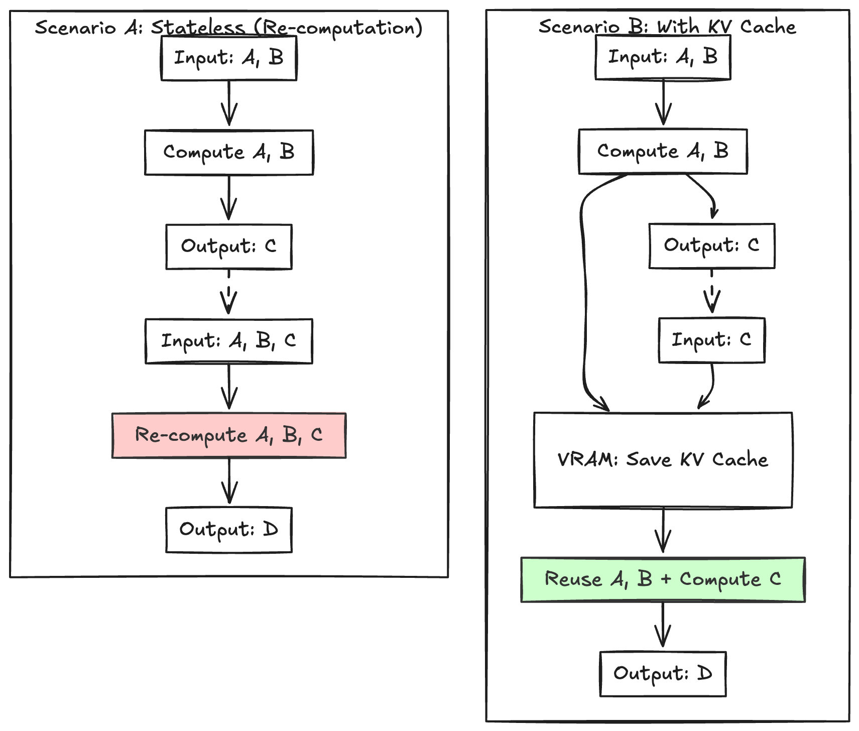
Diagram 1: KV Cache
2. The Architectural Dilemma: To Cache or Not to Cache?
If KV Cache is so fast, why did early cloud APIs (like standard vLLM deployments) often choose to re-compute everything for every request?
The answer lies in Distributed System Design.
The Stateless Approach (Re-computation)
- In this architecture, the Load Balancer routes requests randomly (Round Robin).
- Pros: The system is Stateless. Any GPU can handle any request. Scaling up/down is easy. If a GPU dies, another one takes over instantly.
- Cons: High Latency. Every request must rebuild the “Lego tower” from scratch. This burns GPU compute and increases TCO (Total Cost of Ownership).
The Stateful Approach (Sticky Routing)
- In this architecture, the Load Balancer must send User A’s request to the exact same GPU that holds User A’s cache.
- Pros: Low Latency. We reuse the work we already did.
- Cons: Load Imbalance. What if User A sends a huge request while User B does nothing? The specific GPU handling User A gets overwhelmed, while others sit idle.
Verdict: For short conversations (< 4k tokens), re-computation is acceptable. But for Agentic workflows or RAG (Retrieval Augmented Generation) with 100k+ context, re-computation is impossibly slow.
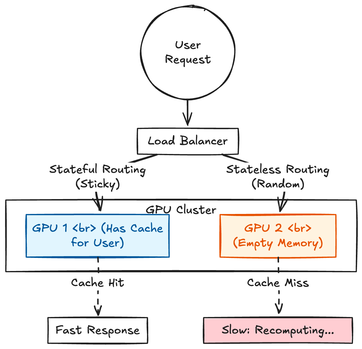
Diagram 2: The Routing Trade-off
3. The Solution: Radix Attention (SGLang)
This is where SGLang changes the paradigm.
Instead of binding a cache to a specific User, SGLang manages memory like a File System Tree (Radix Tree).
How it works:
- Shared Prefix: Most requests in an Agent workflow share the same “System Prompt” or “Few-shot Examples.”
- Tree Structure: The engine stores these shared prefixes as the root of a tree.
- Automatic Reuse: When a new request comes in, the system checks: “Do we have a node in the memory tree that matches this prefix?”
- If Yes: Reuse the memory block immediately.
- If No: Compute only the new part.
This allows the system to be flexible like a stateless system but efficient like a stateful one.
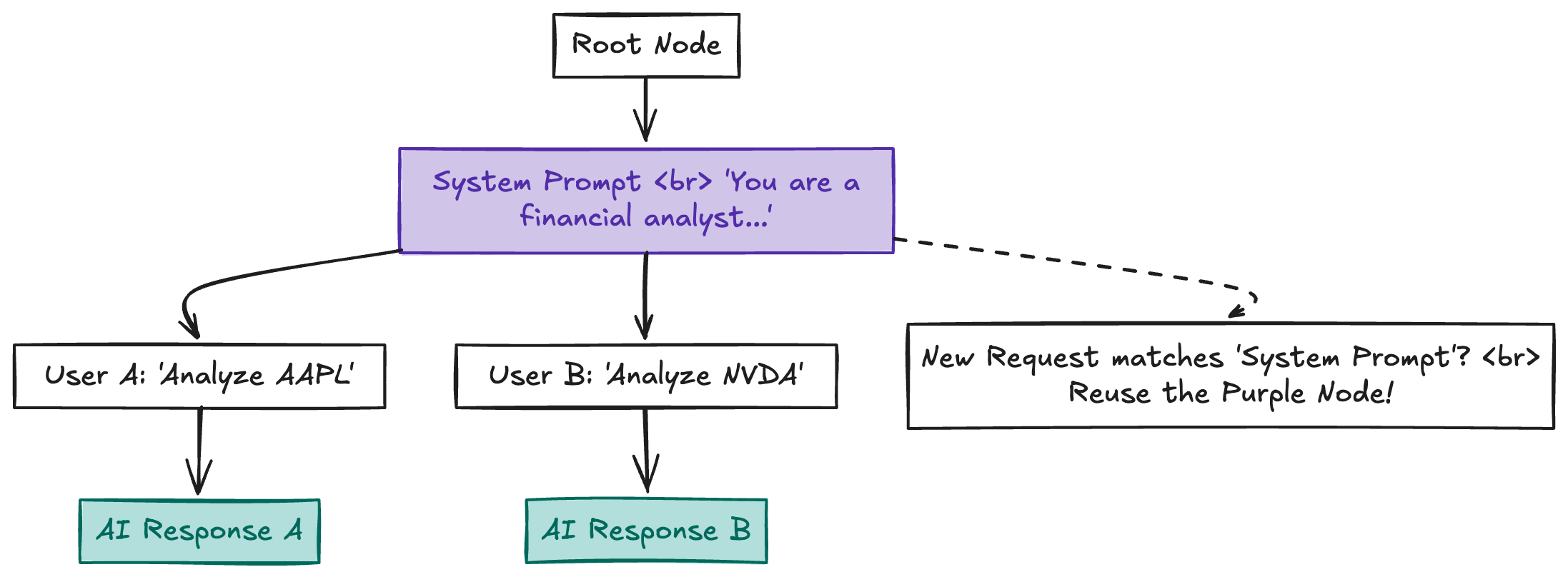
Diagram 3: Radix Attention Structure